

We’ve received a lot of positive feedback since announcing Magic Pocket, our in-house multi-exabyte storage system. We’re going to follow that announcement with a series of technical blog posts that offer a look behind the scenes at interesting aspects of the system, including our protection mechanisms, operational tooling, and innovations on the boundary between hardware and software. But first, we’ll need some context: in this post, we’ll give a high level architectural overview of Magic Pocket and the criteria it was designed to meet.
As we explained in our introductory post, Dropbox stores two kinds of data: file content and metadata about files and users. Magic Pocket is the system we use to store the file content. These files are split up into blocks, replicated for durability, and distributed across our infrastructure in multiple geographic regions.
Magic Pocket is based on a rather simple set of core protocols, but it’s also a big, complicated system, so we’ll necessarily need to gloss over some details. Feel free to add feedback in the comments below; we’ll do our best to delve further in future posts.
Note: Internally we just call the system “MP” so that we don’t have to feel silly saying the word “Magic” all the time. We’ll do that in this post as well.
Requirements
Immutable block storage
Magic Pocket is an immutable block storage system. It stores encrypted chunks of files up to 4 megabytes in size, and once a block is written to the system it never changes. Immutability makes our lives a lot easier.
When a user makes changes to a file on Dropbox we record all of the alterations in a separate system called FileJournal. This enables us to have the simplicity of storing immutable blocks while moving the logic that supports mutability higher up in the stack. There are plenty of large-scale storage systems that provide native support for mutable blocks, but they’re typically based on immutable storage primitives once you get down to the lower layers.
Workload
Dropbox has a lot of data and a high degree of temporal locality. Much of that data is accessed very frequently within an hour of being uploaded and increasingly less frequently afterwards. This pattern makes sense: our users collaborate heavily within Dropbox, so a file is likely to be synced to other devices soon after upload. But we still need reliably fast access: you probably don’t look at your tax records from 1997 too often, but when you do, you want them immediately. We have a fairly “cold” storage system but with the requirement of low-latency reads for all blocks.
To tackle this workload, we’ve built a system based on spinning media (a fancy way of saying “hard drives”), which has the advantage of being durable, cheap, storage-dense and fairly low latency—we save the solid-state drives (SSDs) for our databases and caches. We use a high degree of initial replication and caching for recent uploads, alongside a more efficient storage encoding for the rest of our data.
Durability
Durability is non-negotiable in Magic Pocket. Our theoretical durability has to be effectively infinite, to the point where loss due to an apocalyptic asteroid impact is more likely than random disk failures—at that stage, we’ll probably have bigger problems to worry about. This data is erasure-coded for efficiency and stored across multiple geographic regions with a wide degree of replication to ensure protection against calamities and natural disasters.
Scale
As an engineer, this is the fun part. Magic Pocket had to grow from our initial double-digit-petabyte prototypes to a multi-exabyte behemoth within the span of around 6 months—a fairly unprecedented transition. This required us to spend a lot of time thinking, designing, and prototyping to eliminate the bottlenecks we could foresee. This process also helped us to ensure that the architecture was sufficiently extensible, so we could change it as unforeseen requirements arose.
There were plenty of examples of unforeseen requirements along the way. In one case, traffic grew suddenly and we started saturating the routers between our network clusters. This required us to change our data placement algorithms and our request routing to better reflect cluster affinity (along with available storage capacity, cluster growth schedules, etc) and eventually to change our inter-cluster network architecture altogether.
Simplicity
As engineers we know that complexity is usually antithetical to reliability. Many of us have spent enough time writing complex consensus protocols to know that spending all day reimplementing Paxos is usually a bad idea. MP eschews quorum-style consensus or distributed coordination as much as possible, and heavily leverages points of centralized coordination when performed in a fault-tolerant and scalable manner. There were times when we could have opted for a distributed hash table or trie for our Block Index and instead just opted for a giant sharded MySQL cluster; this turned out to be a really great decision in terms of simplifying development and minimizing unknowns.
Data Model
Before we get to the architecture itself, first let’s work out what we’re storing.
MP stores blocks, which are opaque chunks of files, up to 4MB in size:
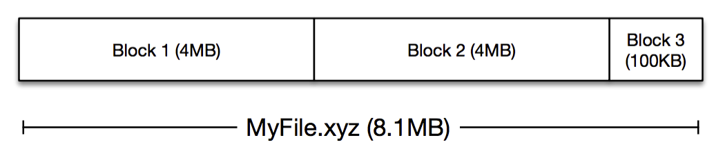
These blocks are compressed and encrypted and then passed to MP for storage. Each block needs a key or name, which for most of our use-cases is a SHA-256 hash of the block.
4MB is a pretty small amount of data in a multi-exabyte storage system however and too small a unit of granularity to move around whenever we need to replace a disk or erasure code some data. To make this problem tractable, we aggregate these blocks into 1GB logical storage containers called buckets. The blocks within a given bucket don’t necessarily have anything in common; they’re just blocks that happened to be uploaded around the same time.
Buckets need to be replicated across multiple physical machines for reliability. Recently uploaded blocks get replicated directly onto multiple machines, and then eventually the buckets containing the blocks are aggregated together and erasure coded for storage efficiency. We use the term volume to refer to one or more buckets replicated onto a set of physical storage nodes.
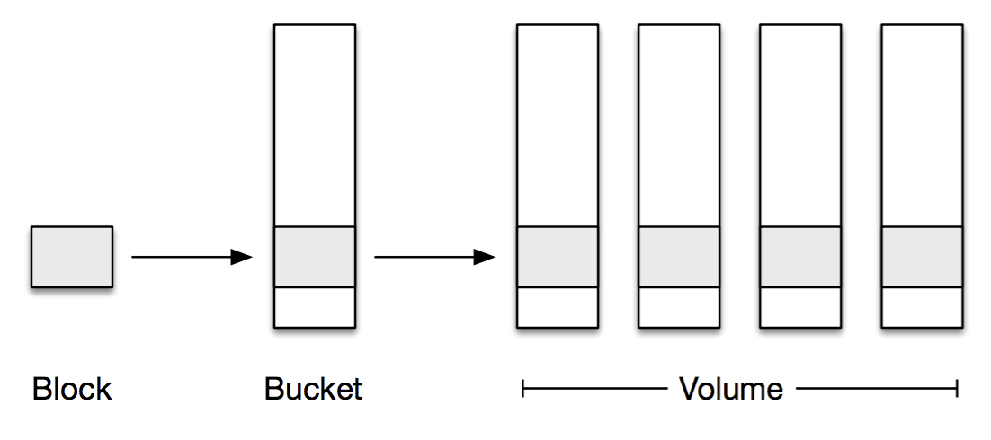
To summarize: A block, identified by its hash, gets written to a bucket. Each bucket is stored in a volume across multiple machines, in either replicated or erasure coded form.
Architecture
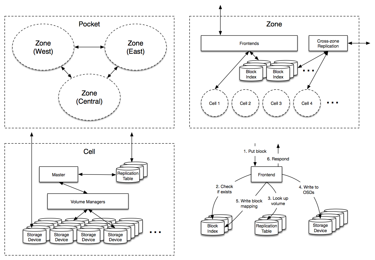
So now that we know our requirements and data model, what does Magic Pocket actually look like? Well, something like this:
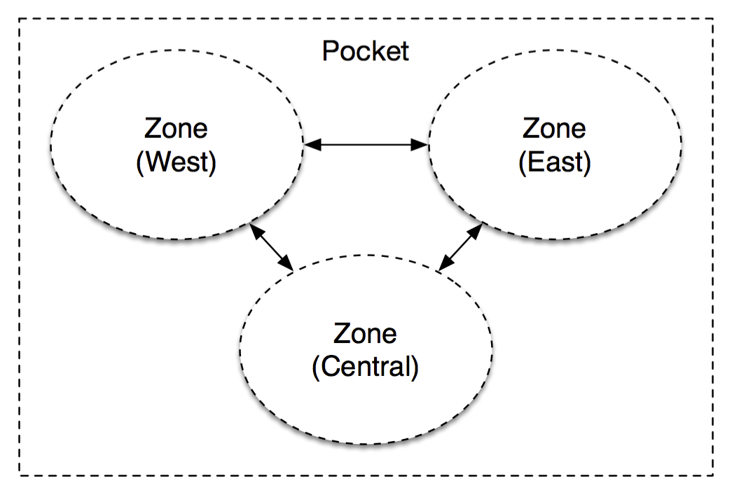
That might not look like much, but it’s important. MP is a multi-zone architecture, with server clusters in western, central and eastern United States. Each block in MP is stored independently in at least two separate zones and then replicated reliably within these zones. This redundancy is great for avoiding natural disasters and large-scale outages but also allows us to establish very clear administrative domains and abstraction boundaries to avoid a misconfiguration or congestion collapse from cascading across zones.
[We have some extensions in the works for less-frequently accessed (“colder”) data that adopts a different multi-zone architecture than this.]
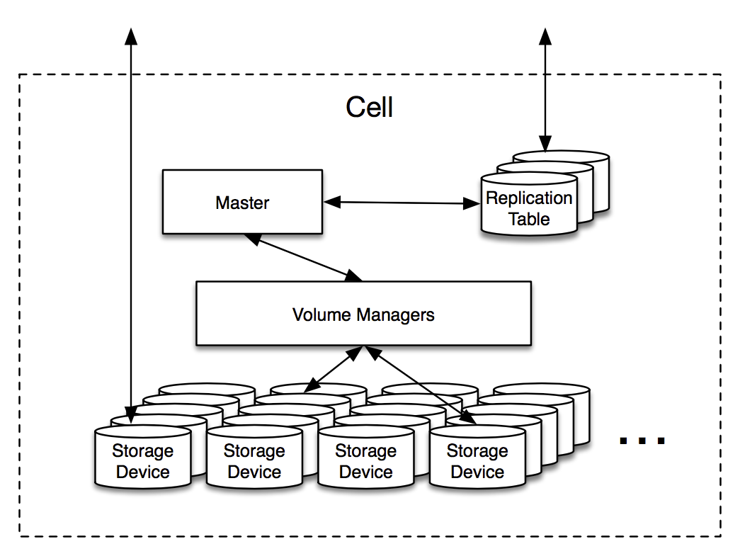
Most of the magic happens inside a zone however, so let’s dive in:
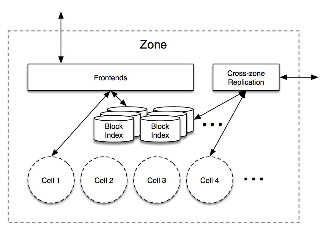
hash → cell, bucket, checksum
bucket → volume
volume → OSDs, open, type, generation
Protocol
Phew! You’ve made it this far, and hopefully have a reasonable understanding of the high-level Magic Pocket architecture. We’ll wrap up with a very cursory overview of some core MP protocols, which we can expound upon in future posts. Fortunately these protocols are already quite simple.
Put
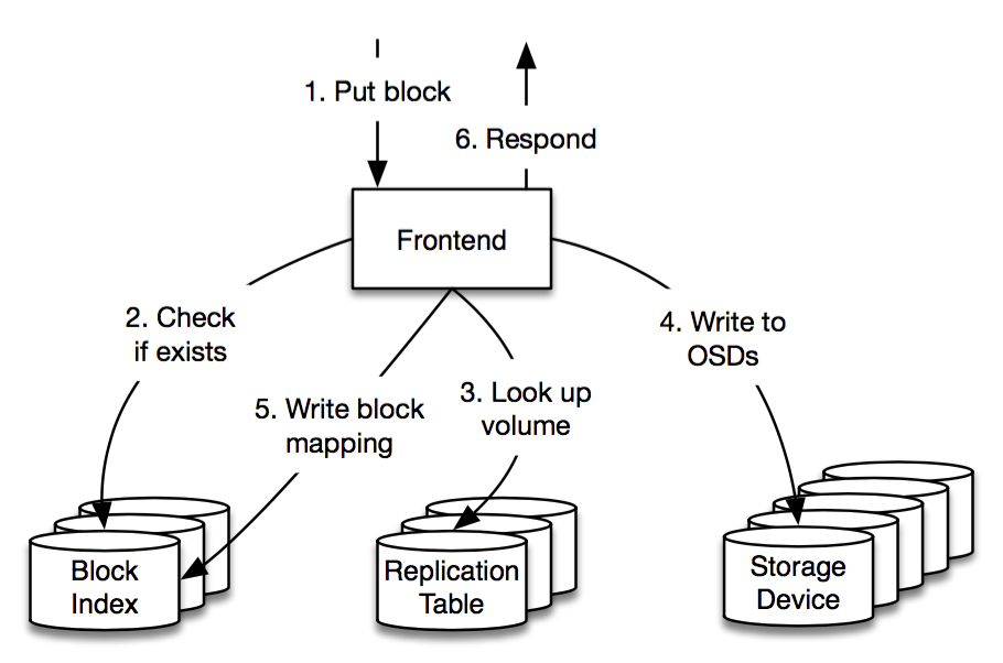
The Frontends are armed with a few pieces of information in advance of receiving a Put request: they periodically contact each cell to determine how much available space it has, along with a list of open volumes that can receive new writes.
When a Put request arrives, the Frontend first checks if the block already exists (via the Block Index) and then chooses a target volume to store the block. The volume is chosen from the cells in such a way as to evenly distribute cell load and minimize network traffic between storage clusters. The Frontend then consults the Replication Table to determine the OSDs that are currently storing the volume.
The Frontend issues store commands to these OSDs, which all fsync the blocks to disk (or on-board SSD) before responding. If this was successful then the Frontend adds a new entry to the Block Index and can return successfully to the client. If any OSDs fail along the way then the Frontend just retries with another volume, potentially in another cell. If the Block Index fails then the Frontend forwards the request to the other zone. The Master periodically runs background tasks to clean up from any partial writes for failed operations.
There are some subtle details behind the scenes, but ultimately it’s rather simple. If we adopted a quorum-based protocol where the Frontend was only required to write to a subset of the OSDs in a volume then we would avoid some of these retries and potentially achieve lower tail latency but at the expense of greater complexity. Judicious management of timeouts in a retry-based scheme already results in low tail latencies and gives us performance that we’re very happy with.
Get
Once we know the Put protocol, the process for serving a Get should be self-explanatory. The Frontend looks up the cell and bucket from the Block Index, then looks up the volume and OSDs from the Replication Table, and then fetches the block from one of the OSDs, retrying if one is unavailable.
As mentioned, we store both replicated data and erasure coded data in MP. Reading from a replicated volume is easy because each OSD in the volume stores all the blocks.
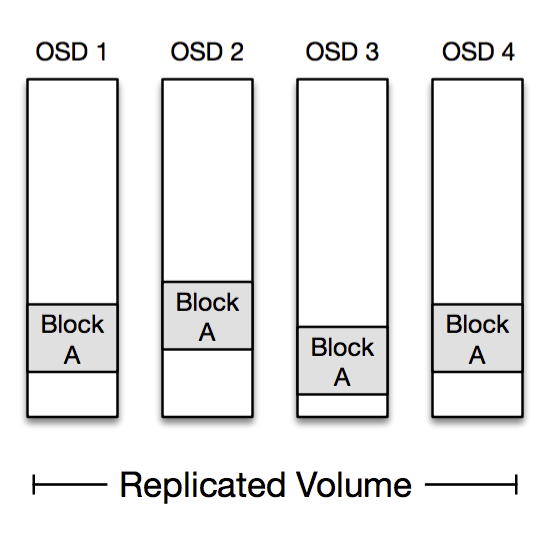
Reading from an erasure coded volume can be a little more tricky. We encode in such a way that each block can be read in entirety from a single given OSD, so most reads only hit a single disk spindle; this is important in reducing load on our hardware. If that OSD is unavailable then the Frontend needs to reconstruct the block by reading encoded data from the other OSDs. It performs this reconstruction with the aid of the Volume Manager.
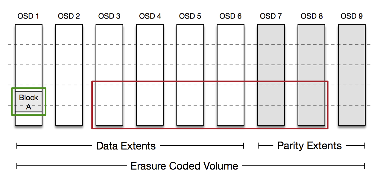
In the encoding scheme above, the Frontend can read Block A from OSD 1, highlighted in green. If that read fails it can reconstruct Block A by reading from a sufficient number of blocks on the other OSDs, highlighted in red. Our actual encoding is a little more complicated than this and is optimized to allow reconstruction from a smaller subset of OSDs under most failure scenarios.
Repair
The Master runs a number of different protocols to manage the volumes in a cell and to clean up after failed operations. But the most important operation the Master performs is Repair.
Repair is the operation used to re-replicate volumes whenever a disk fails. The Master continually monitors OSD health via our service discovery system and triggers a repair operation once an OSD has been offline for 15 minutes — long enough to restart a node without triggering unnecessary repairs, but short enough to provide rapid recovery and minimize any window of vulnerability.
Volumes are spread somewhat-randomly throughout a cell, and each OSD holds several thousand volumes. This means that if we lose a single OSD we can reconstruct the full set of volumes from hundreds of other OSDs simultaneously:
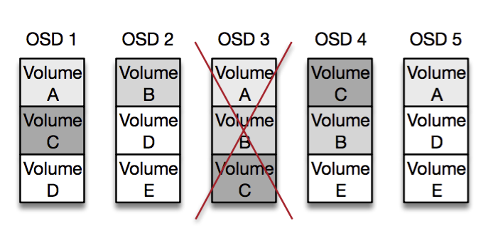
In the diagram above we’ve lost OSD 3, but can recover volumes A, B and C from OSDs 1, 2, 4 and 5. In practice there are thousands of volumes per OSD, and hundreds of other OSDs they share this data with. This allows us to amortize the reconstruction traffic across hundreds of network cards and thousands of disk spindles to minimize recovery time.
The first thing the Master does when an OSD fails is to close all the volumes that were on that OSD and instruct the other OSDs to reflect this change locally. Now that the volumes are closed, we know that they won’t accept any future writes and are thus safe to move around.
The Master then builds a reconstruction plan, where it chooses a set of OSDs to copy from and a set of OSDs to replicate to, in such a way as to evenly spread load across as many OSDs as possible. This step allows us to avoid traffic spikes on particular disks or machines. The reconstruction plan allows us to provision far fewer hardware resources per OSD, and would be difficult to produce without having the Master as a central point of coordination.
We’ll gloss over the data transfer process, but it involves the volume managers copying data from the sources to the destinations, erasure coding where necessary, and then handing control back to the Master.
The final step is fairly simple, but critical: At this point the volume exists on both the source and destination OSDs, but the move hasn’t been committed yet. If the Master fails at this point, the volume will just stay in the old location and get repaired again by the new Master. To commit the repair operation, the Master first increments the generation number on the volumes on the new OSDs, and then updates the Replication Table to store the new volume-to-OSD mapping with the new generation (the commit point). Now that we’ve incremented the generation number we know that there’ll be no confusion about which OSDs hold the volume, even if the failed OSD comes back to life.
This protocol ensures that any node can fail at any time without leaving the system in an inconsistent state. We’ve seen all sorts of crazy stuff in production. In one instance, a database frontend froze for a full hour before springing back to life and forwarding a request to the Replication Table, during which time the Master had also failed and restarted, issuing an entirely different set of repair operations. Our consistency protocols need to be completely solid in the face of arbitrary failures like these. The Master also runs a number of other background processes such as Reconcile, which validates OSD state and rolls back failed repairs or incomplete operations.
The open/closed volume model is key for ensuring that live traffic doesn’t interfere with background operations, and allows us to use far simpler consistency protocols than if we didn’t enforce this dichotomy.
Wrap-up
Thanks for making it this far! Hopefully this post gives some context for how Magic Pocket works and for some of our motivations.
The primary design principle here is keep it simple! Designing a distributed storage system is a big challenge, but it’s much harder to build one that operates reliably at scale, and supports all of the monitoring and verification systems and tooling that will ensure it’s running correctly. It’s also incredibly important to make technical decisions that are the right solution to the right problem, not just because they’re cool and novel. Most of MP was built by a team of less than half a dozen people, which required us to focus on the things that mattered, and played a big part in the success of the project.
There are obviously a lot of details that we’ve left out. (Just in case you’re about to respond, “Wait! this doesn’t work when X, Y and Z happens!”—we’ve thought about that, I promise.) Stay tuned for future blog posts where we’ll go into more detail on specific aspects about building and operating a system at this scale.


