

Document scanning as augmented reality
Dropbox's document scanner shows an overlay of the detected document over the incoming image stream from the camera. In some sense, this is a rudimentary form of augmented reality. Of course, this isn't revolutionary; many apps have the same form of visualization. For instance, many camera apps will show a bounding box around detected faces; other apps show the world through a color filter, a virtual picture frame, geometric distortions, and so on.
One constraint is that the necessary processing (e.g., detecting documents, detecting and recognizing faces, localizing and classifying objects, and so on) does not happen instantaneously. In fact, the fancier one's algorithm is, the more computations it needs and the slower it gets. On the other hand, the camera pumps out images at 30 frames per second (fps) continuously, and it can be difficult to keep up. Exacerbating this is the fact that not everyone is sporting the latest, shiniest flagship device; algorithms that run briskly on the new iPhone 7 will be sluggish on an iPhone 5.
We ran into this very issue ourselves: the document detection algorithm described in our earlier blog post could run in real-time on the more recent iPhones, but struggled on older devices, even after leveraging vectorization (performing many operations simultaneously using specialized hardware instructions) and GPGPU (offloading some computations to the graphics processor available on phones). In the remaining sections, we discuss various approaches for reconciling the slowness of algorithms with the frame rate of the incoming images.
Approach A: Asynchronous Processing
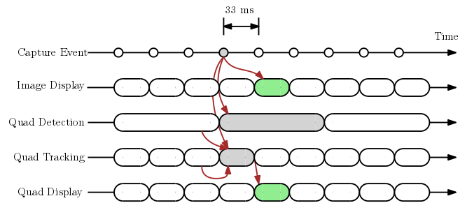
Let’s assume from here on that our document detection algorithm requires 100ms per frame on a particular device, and the camera yields an image every 33 ms (i.e., 30 fps). One straightforward approach is to run the algorithm on a “best effort” basis while displaying all the images, as shown in the diagram below.
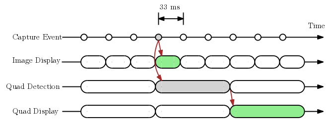
The diagram shows the relative timings of various events associated with a particular image from the camera, corresponding to the “Capture Event” marked in gray. As you can see, the image is displayed for 33 ms (“Image Display”) until the next image arrives. Once the document boundary quadrilateral is detected (“Quad Detection”), which happens 100 ms after the image is received, the detected quad is displayed for the next 100 ms (“Quad Display”) until the next quad is available. Note that in the time the detection algorithm is running, two more images are going to be captured and displayed to the user, but their quads are never computed, since the quad-computing thread is busy.
The major benefit of this approach is that the camera itself runs at its native speed—with no external latency and at 30 fps. Unfortunately, the quad on the screen only updates at 10 fps, and even worse, is offset from the image from which it is computed! That is, by the time the relevant quad has been computed, the corresponding image is no longer on screen. This results in laggy, choppy quads on screen, even though the images themselves are buttery smooth, as shown in the animated GIF below.
Approach B: Synchronous Processing
In contrast to the first approach, the major benefit here is that the quad will always be synced to the imagery being displayed on the screen, as shown in the first animated GIF below.
Unfortunately, the camera now runs at reduced frame rate (10 fps). What's more disruptive, however, is the large latency (100 ms) between the physical reality and the viewfinder. This is not visible in the GIF alone, but to a user who is looking at both the screen and the physical document, this temporal misalignment will be jarring and is a well-known issue for VR headsets.
Approach C: Hybrid Processing
The two approaches described thus far have complementary strengths and weaknesses: it seems like you can either get smooth images OR correct quads, but not both. Is that true, though? Perhaps we can get the best of both worlds?
A good rule of thumb in performance is to not do the same thing twice, and this adage applies aptly in video processing. In most cases, camera frames that are adjacent temporally will contain very similar data, and this prior can be exploited as follows:
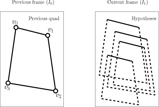
- If we detected a quad containing vertices {v0, v1, v2, v3} in a camera frame I0, the quad to be found in the next camera frame I1 will be very similar, modulo the camera motion between the frames.
- If we can figure out what kind of motion T occurred between the two camera frames, we can apply the same motion to the quad in the first frame, and we will have a good approximation for the new quad, namely {T(v0), T(v1), T(v2), T(v3)}.
While this is a promising simplification that turns our original detection problem into a tracking problem, robustly computing the transformation between two images is a nontrivial and slow exercise on its own. We experimented with various approaches (brute-forcing, keypoint-based alignment with RANSAC, digest-based alignment), but did not find a satisfactory solution that was fast enough.
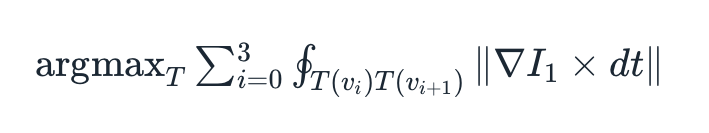
In fact, there is an even stronger prior than what we claimed above; the two images we are analyzing are not just any two images! Each of these images, by stipulation, contains a quad, and we already have the quad for the first image. Therefore, it suffices to figure out where in the second image this particular quad ends up. More formally, we try to find the transform of this quad such that the edge response of the hypothetical new quad, defined to be the line integral of the gradient of the image measured perpendicular to the perimeter of the quad, is maximized. This measure optimizes for strong edges across the boundaries of the document.
See the appendix below for a discussion on how to solve this efficiently.
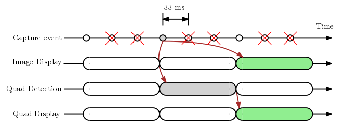
Theoretically, we could now run detection only once and then track from there on out. However, this would cause any error in the tracking algorithm to accumulate over time. So instead, we continue to run the quad detector as before, in a loop—it will now take slightly over 100 ms, given the extra compute we are performing—to provide the latest accurate estimate of the quad, but also perform quad tracking at the same time. The image is held until this (quick) tracking process is done, and is displayed along with the quad on the screen. Refer to the diagram below for details.
In summary, this hybrid processing mode combines the best of both asynchronous and synchronous modes, yielding a smooth viewfinder with quads that are synced to the viewfinder, at the cost of a little bit of latency. The table below compares the three methods:
| Asynchronous | Synchronous | Hybrid | |
| Image throughput | 30 Hz | 10 Hz | 30 Hz |
| Image latency | 0 ms | 100 ms | ~30 ms |
| Quad throughput | 10 Hz | 10 Hz | 30 Hz |
| Quad latency | 100 ms | 100 ms | ~30 ms |
| Image vs quad offset | 100 ms | 0 ms | 0 ms |
The GIF below compares the hybrid processing (in blue) and the asynchronous processing (in green) on an iPhone 5. Notice how the quad from the hybrid processing is both correct and fast.
Appendix: Efficiently localizing the quad
In practice, we observed that the most common camera motions in the viewfinder are panning (movement parallel to the document surface), zooming (movement perpendicular to the document surface), and rolling (rotating on a plane parallel to the document surface.) We rely on the onboard gyroscope to compute the roll of the camera between consecutive frames, which can then be factored out, so the problem is reduced to that of finding a scaled and translated version of a particular quadrilateral.
In order to localize the quadrilateral in the current frame, we need to evaluate the aforementioned objective function on each hypothesis. This involves computing a line integral along the perimeter, which can be quite expensive! However, as shown in the figure below, the edges in all hypotheses can have only one of four possible slopes, defined by the four edges of the previous quad.
Exploiting this pattern, we precompute a sheared running sum across the entire image, for each of the four slopes. The diagram below shows two of the running sum tables, with each color indicating the set of pixel locations that are summed together. (Recall that we sum the gradient perpendicular to the edge, not the pixel values.)
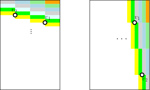
Once we have the four tables, the line integral along the perimeter of any hypothesis can be computed in O(1): for each edge, look up the running sums at the endpoints in the corresponding table, and calculate the difference in order to get the line integral over the edge, and then sum up the differences for four edges to yield the desired response. In this manner, we can evaluate the corresponding hypotheses for all possible translations and a discretized set of scales, and identify the one with the highest response. (This idea is similar to the integral images used in the Viola-Jones face detector.)


