

We introduced Cape in a previous post. In a nutshell, Cape is a framework for enabling real-time asynchronous event processing at a large scale with strong guarantees. It has been over a year since the system was launched. Today Cape is a critical component for Dropbox infrastructure. It operates with both high performance and reliability at a very large scale. Here are a few key metrics, Cape is:
- running on thousands of servers across the continent
- subscribing to over 30 different event domains at a rate of 30K/s
- processing jobs of various sizes at rate of 150K/s
- delivering 95% of events under 1 second after they are created.
Cape has been widely adopted by teams at Dropbox. Currently there are over 70 use cases registered under Cape’s framework, and we expect Cape adoption to continue to grow in the future.
In this post, we’ll take a deep dive into the design of the Cape framework. First, we’ll discuss Cape’s architecture. Then we’ll look at the core scheduling component of the system. Throughout, we’ll focus the discussion on a few key design decisions.
Design principles behind Cape
Before we begin, let’s touch on a few of our principles for developing and maintaining Cape. These principles were proposed based on learnings from the development of other systems at Dropbox, especially from Cape’s predecessor Livefill. These principles were critical for both the project’s success and the ongoing maintenance of the system.
Modularization From the beginning we explicitly took a modular approach to system design; this is critical for isolating complexities. We created modules with clearly defined functionalities, and carefully designed the communication protocols between these modules. This way, when building a module we only needed to worry about a limited number of issues. Testing was easy since we could verify each module independently. We also want to highlight the importance of keeping module interface to a minimum. It’s easier to reason about interaction between the modules when their interfaces are small. What’s more, a small interface is more easily adapted to new use cases.
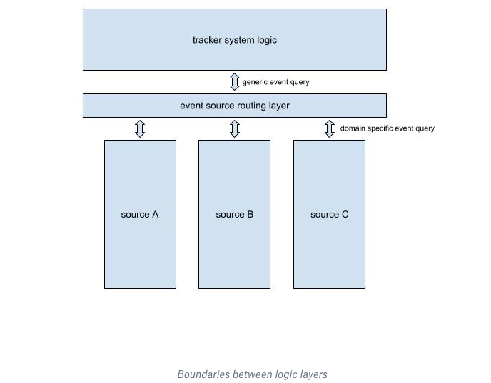
Clear boundaries between system logic and application-specific logic In Cape it’s common for a component to contain procedures for both system logic and application-specific logic. For instance, the dispatcher’s tracker queries information from the event source (application specific), and produces scheduling requests based on query results (system logic).
We carefully designed Cape’s abstraction to ensure there is a clear boundary between the two categories. As illustrated in the following figure, system logic and application specific query logic are separated by an intermediate layer. It translates generic queries issued by the tracker into specific queries to different event sources. This boundary ensures that the system is easily extensible, and that logic for different event sources is completely isolated.
Evolution of terminology
The following terms and concepts are necessary for understanding the fundamentals of how Cape functions. During the course of Cape's development, definitions for the following key terms and concepts evolved and became further refined. Readers may wish to re-read the previous post for a refresh. Otherwise, a quick recap will promote the following discussion.
In Cape’s world, an event is a piece of persisted data. The key for any event has two components. One component is a subject, of type string. The second component is sequence ID, of type integer. Events with the same subject are ordered by their sequence IDs, and those with different subjects are considered independent. A namespace for events that are constructed in the same way is a domain.
Topology is our notion of a user application. Topologies that subscribe to the same domains can form ordering dependencies. In other words, users can specify a set of other topologies that must run before their own topologies do.
Lambdas carry out execution. Conceptually, lambdas are callbacks that are invoked with a set of events provided as input. Going back to topology, a topology consists of one or more lambdas. Within the scope of a topology, lambdas may form data dependency. This means a lambda can generate output regarding an event, and the output will become input for one or more other lambdas when processing the same event. Why have multiple lambdas carry out a topology’s logic? At Dropbox one popular motivation is data vicinity. If a topology’s workflow can be divided into stages that process data in different datacenters, then it’s more efficient to colocate the computation with data. In this case a user may choose to have multiple lambdas running in different data centers.
For each subject's topology, we maintain the sequence ID of the last successfully processed event. This value is called a cursor. All the cursors of a single subject are included in one protobuf object, which we call cursor info. Cursor info is persisted and can be retrieved with the subject as key.
Architecture: why not just a queue?
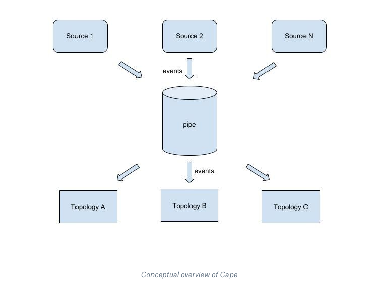
Cape is an event delivery system. Conceptually, it can be thought of as a pipe, as below. At one end event sources notify Cape of new events. At the other end events are consumed by various topologies.
A queue-based solution isn’t enough to meet requirements
Cape’s event-processing design is result of the following requirements for how events should be delivered:
- low latency: events should be delivered as fast as possible
- retry until success: each event is guaranteed to be eventually successfully processed by all subscribing topologies
- subject level isolation: failures in one subject shouldn’t impact the processing of events from other subjects
- event source reliability: event sources are external services and therefore they can fail from time to time. The system must be able to tolerate failures such as when sources fail to send out events.
Although a queue is the natural solution for event delivery, if we take the above requirements into consideration, it quickly becomes apparent that a queue-based solution isn’t enough.
Imagine building a queue-based system that satisfies Cape’s requirements. For simplicity, we’ll limit our discussion to a few common and mature solutions for queues: Kafka, Redis, and SQS. Queue-based solutions require event sources to reliably push each event to the system. Additionally, events are pushed with correct ordering, meaning that for the same subject, events with smaller sequence IDs are pushed first. Now let’s go through some of the above requirements.
Low latency
Comparatively speaking, publishing to Kafka is significantly faster than SQS. Kafka is designed for low latency publishing. We can set up Kafka clusters in Dropbox infrastructure, so its network latency is going to be much lower than using SQS.
Redis has very low latency when data is only in memory. However when it’s configured to persist snapshot data, there can be significant negative impact on its availability.
Retry until success
In a queue-based solution, this is equivalent to a requirement for persistency. Both Kafka and SQS support data persistency very well.
For Redis, as mentioned above, persistency can be achieved to some extent by taking periodic snapshots, which impacts availability. Additionally, a Redis cluster with persisted data is usually more difficult to maintain compared to Kafka or SQS.
Subject level isolation
Subject level isolation is the biggest barrier to queueing. It’s not practical to create a queue for each subject; there can be billions of them. The problem with using Kafka for queuing is that Kafka requires each consumer to acknowledge each event after it’s been successfully processed. This introduces a severe head-of-the-line blocking problem because it prevents processing any other subjects’ events until the one at the head of the queue is successfully processed. The latency is unacceptable—there are thousands of subjects generating events every second, and lambda runtime can vary from milliseconds to tens of minutes.
Delivery latency could be improved by decoupling an event’s read and acknowledgement phases. This would allow consumers to keep reading new events while asynchronously acknowledging them after successful processing. But, if any event misses getting processed the consumer will have to rewind and reprocess a potentially large amount of other subjects’ events. This rewind is necessary to provide an “at least once” success guarantee for every event. Essentially, failure in one subject can introduce duplicated processing and extra latency to other subjects, which breaks the isolation between subjects.
SQS provides a better solution for this kind of isolation. When an event is being consumed it is invisible to other consumers, until a specified deadline is reached. Once successful processing has finished the consumer acknowledges it and the event is removed from the queue. This allows consumers to keep fetching new events, without having to worry about rewind on failures.
However, with SQS there is a problem when ordered processing is taken into consideration. Although it has a first-in, first out (FIFO) option that provides ordered consumption, it comes at the cost of limited throughput. Otherwise the problem is that, before processing an event, there is no way for a consumer to know whether an event’s predecessors were successfully processed. Without knowing that, guarantees of ordered processing cannot be made. Complicating the issue, a record indicating which consumer gets the right to exclusively process which subject would have to be made (to ensure events of the same subjects are processed in order). This kind of bookkeeping can be tricky to maintain and we would need to build the service for necessary bookkeeping.
The requirement for subject level isolation is also problematic when using Redis for queuing. In practice, consuming an event from Redis means removing it from the queue. This creates a durability issue. The event will be lost if the consumer crashes, a very common event. While it’s possible to let the consumer peek at the event and only remove it after it’s successfully processed, that also leads to a head-of-the-line blocking problem, and it doesn’t solve the issue of lost events.
Event source reliability
Finally we come back to the initial setup: events must be published by the source in a reliable way. In production this can be very hard to achieve. Often the creation of an event is in the path of a critical Dropbox service (think about syncing a file or signing up as new user). In a large scale distributed system, failure happens almost all the time. When there is a publish failure, the rational choice is to give up so as to avoid impacting the critical service’s availability. The event goes unpublished.
Why build a dispatcher?
Given the above discussion, using SQS plus a bookkeeping service could provide a possible queuing solution, but we still needed to address scalability and reliability. Because the queue-based system isn’t reliable, and the inefficiency entailed in custom bookkeeping would make scaling a difficult prospect, we chose to build Cape’s scheduling component with a dispatcher.
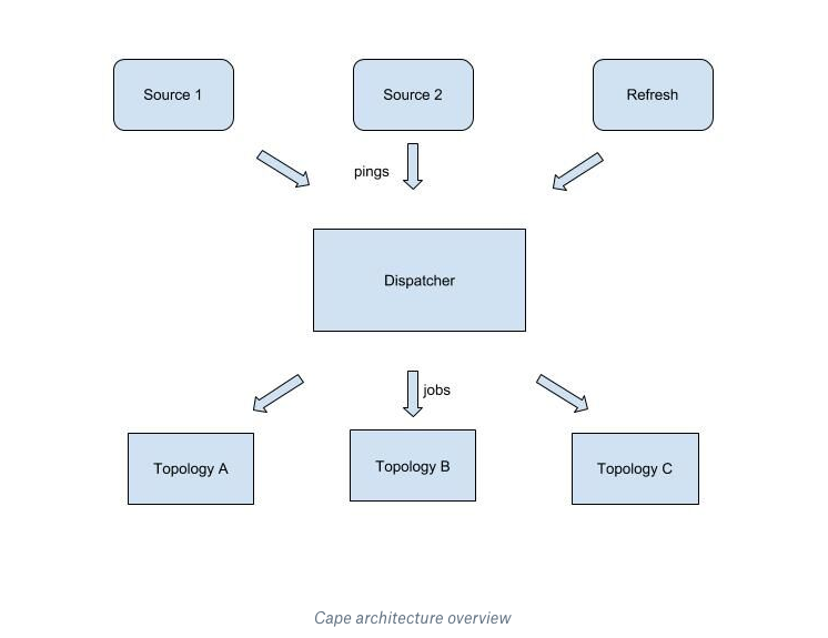
Rather than having event sources send every event with proper ordering to a queue, event sources send pings to a dispatcher. This setup imposes much less workload on event sources as the publish workload for event sources is significantly smaller. Since the Cape has a refresh feature, all pings get tried at least once. Lastly, because all scheduling operations happen inside the dispatcher (avoiding slow communication between servers), we can achieve very low event delivery latency. As a side benefit, having a centralized scheduling component allows Cape to support more advanced processing modes, including scheduling with dependency, ordered processing, and heartbeat.
Dispatcher Overview
The dispatcher lies at center of Cape’s architecture. It is the system’s brain and controls the full lifecycle of scheduling. Let’s first take a look at dispatcher at the top level. The dispatcher’s data flow is summarized in the following figure.
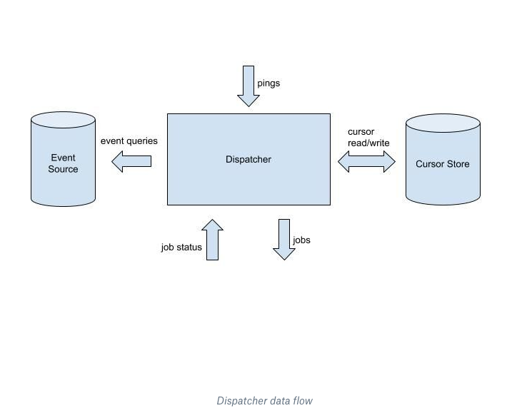
Event sources send lightweight, subject-related pings to the dispatcher. The ping reminds the dispatcher to check and see whether there are any new events to be processed for that subject. Upon receiving the ping, the dispatcher makes a few queries to gather relevant information. This includes querying the cursor from the cursor store, and getting event information from the sources. Using these query results, the dispatcher updates its in-memory state and determines which events need to be processed by which lambdas. At this point jobs—a set of events and a unique job ID—are issued to the corresponding lambda workers.
After a worker finishes the processing, it reports back to the dispatcher with a job status. This contains the process results for each event and the same job ID for the corresponding job. Upon receiving job status results, the dispatcher updates the in-memory state. If the job was a success, the dispatcher may advance the corresponding cursor and schedule more jobs if any new scheduling can be triggered. The scheduling lifecycle for a ping ends when the dispatcher’s in-memory state doesn’t have any records for running jobs, and there are no more jobs to be issued. An important feature is the ping refresh component. When pings can’t make it to the dispatcher, Cape’s refresh feature will make sure to resend any lost pings.
Dispatcher internal structures
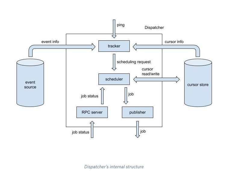
Above is a graph of the dispatcher’s internal process. A highlight of the dispatcher design is modularity, one of the key design principles we started with. Each component carries out relatively independent functionality. Instead of sharing memory state, components coordinate with each other by passing messages, though the communication protocol between components is minimal. This design allows each component to be tested separately with great ease.
Tracker
The tracker is a stateless component that receives pings as input, and produces one or more scheduling requests for the scheduler to consume. It queries the cursor store and event sources for information necessary to making scheduling decisions, and then compiles scheduling requests. Of all the data inside a request, the most important pieces are event interval and event set. The event interval is a closed interval of sequence IDs, and the event set contains all the events within the corresponding interval.
Scheduler
The scheduler is the only stateful component inside the dispatcher and is the only entity that can write to the cursor store in Cape. Except for reading and writing cursors, the scheduler’s operations are all strictly in memory. Additionally, the scheduler owns the in-memory state that keeps the bookkeeping for jobs.
When the scheduler gets a request it creates new jobs and sends them out to the publisher—a stateless component that receives jobs. It sends jobs to an external buffer which is subscribed to by corresponding lambda workers. The RPC server gets the job status from the workers and forwards it to the scheduler. Depending on success or failure, the scheduler may issue more jobs. Because it’s the only component that owns in-memory state, it does all the related bookkeeping.
This reflects our observation of scheduling operations. Every scheduling operation consists of expensive but stateless remote queries, plus in-memory logic that requires locking. In our design, stateless procedures are managed by peripheral components and the scheduler focuses on almost pure in-memory scheduling procedures. Components run in parallel and communicate by sending messages. This provides a clear view of how different components work together and the implementation for parallelism is straightforward because the design naturally fits Go’s concurrency model.
Deep Dive into two important elements
Two key elements that deserve a deeper look are tracker’s procedure for scheduling requests, and the scheduler data structures and algorithm.
Tracker operation
The tracker takes a ping as input and produces one or more scheduling requests as output. A scheduling request is an object packed with all the information necessary for making scheduling decisions, including:
- the subject’s latest sequence ID
- the event interval [sequenceId_start, sequenceId_target]
- a set of all events within the above interval
This tracker procedure is best demonstrated with an example. Let’s say a ping regarding subject S is received, and there are 4 topologies: T1–T4, subscribing to subject S’s events. Upon receiving this ping, the tracker first queries the latest sequence ID for S, which is 100. Then it queries S’s cursor info. Let’s say the content of the cursor info is:
- T1: 10
- T2: 90
- T3: 99
- T4: 99
Next, the tracker needs to make event queries in order to fetch events for scheduling. An event query takes three arguments: subject, start sequence ID, and max batch size. It returns a sorted list of events beginning with the start sequence ID and which is capped in length by a max batch size. The max batch size is set based on the capability of the event source, as well as on the data size per event from this source. In this example let’s assume the limit is 10. Additionally, it’s important to note that for a given topology, an event range can be used to create new jobs for the topology only when the range contains the topology’s cursor + 1.
As you can imagine, event queries can be very expensive, both in terms of latency and the load on the event source. This creates an interesting optimization problem: how do you make the minimum number of event queries, and still allow all topologies to make as much progress as possible?
The most naive approach would be to make an event query for each topology. But the problem with this approach is also obvious: it doesn’t scale. As more topologies subscribe to the same event source, the tracker’s workload grows linearly. Because the topologies’ cursors are nearly aligned most of the time, most of the tracker’s queries will be redundant.
For our first iteration, we adopted a simple heuristic: make one event query for each distinct cursor value. For instance in the above setting, tracker will make three queries with the following arguments:
- (S, 11, 10)
- (S, 91, 10)
- (S, 100, 10)
This had very good performance in the beginning, when most topologies had very simple and robust processing logic. However, as we started adding expensive topologies with jobs that take longer time to execute, or that were sometimes flaky with errors, we observed the system frequently fell into an unstable state where the dispatcher was running hot on CPU and couldn’t keep up with the scheduling.
A thorough investigation revealed that the problem was with the event query heuristic. It works well when most topologies have their cursor values aligned. However once a few of them start to experience increased failures, more and more distinct cursor values emerge for a single subject. This causes the tracker’s worker pool to become increasingly busy and then scheduling gets delayed or canceled as the system approaches its capacity limit. This is a vicious cycle. Once the system becomes overwhelmed things only get worse. The system cannot recover on its own.
Given that the first heuristic wasn’t robust, an improved heuristic was proposed and applied. In this new approach, cursor values are grouped by vicinity. Only one event query is made for a group. This an improvement because it generates fewer requests than first heuristic when some topologies are degraded. For the given example, we only generate the following event queries:
- (S, 11, 10)
- (S, 91, 10)
This heuristic has much better tolerance on small cursor misalignment, and is much more robust. When a few topologies are behaving badly, their impact on the dispatcher is well constrained. This heuristic also proved to be highly scalable. We added tens of topologies for a particular event domain, and Cape continues to run efficiently, with very high stability.
Scheduler: the only stateful component in Cape’s system
Now let’s talk about the scheduler. The scheduler exclusively owns the dispatcher’s in memory data structure for bookkeeping jobs that are currently inflight. For this reason, we call this data structure inflight state. When new information is received from either the tracker or the RPC server, the scheduler updates the inflight state accordingly, and makes correct scheduling decisions.
Now we’ll look at inflight state and an illustration of how the scheduling algorithm works. First, a look at the basic scheduling workflow.
Inflight state: The inflight state has three components. The first component is a tree structure that allows scheduling information to be stored hierarchically, it’s called state tree. Nodes at the first level of state tree are called subject state. They are the root of the subtree that contains all inflight information for a given subject. Information shared by all inflight jobs for this subject, including cursor info, latest sequence ID, and the ranges of events used by the subject’s inflight jobs are stored by the subject state node. The subject state fans out to the topology state. It’s the root of the subtree that corresponds to this topology’s inflight jobs. Finally, the leaf node is the lambda state, containing a sorted list of the inflight job records.
The following graph shows the layout of the state tree. Note how at the root level there is a subject state table that maps inflight subjects to their corresponding subject state nodes.
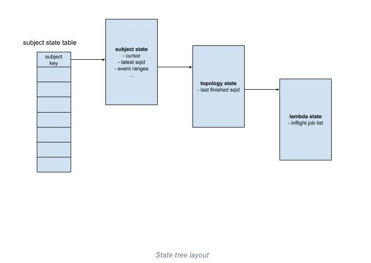
The second component is a timeout list. It’s a priority queue holding references to all inflight jobs, as sorted by their expiration timestamps. A job lookup table, keyed by job ID, is the third component. It maintains the job metadata, which is used to find corresponding job records in the timeout list and the state tree.
Scheduling algorithm: To show how the scheduling algorithm works, we need to set up some necessary context. Let’s first assume there are two topologies, T1 and T2. Both subscribe to the same event domain. For simplicity, we’ll assume they both contain a single lambda. The scheduler has received a scheduling request with the following content:
- subject: S
- latest sequence ID: 100
- event interval: [91, 100]
- event set: [91, 99, 100] (note that sequence IDs might not be consecutive)
Upon receiving this request, the scheduler initiates a scheduling procedure that is carried out by a Go routine. The scheduling procedure finds all the relevant lambda states in the state tree and tries to generate new jobs inside those state nodes. The procedure begins from the subject state. At root there is a table that maps subjects to a corresponding subject state. However, before making any attempts to access a subject state, a lock for that particular subject must be held. This guarantees that no race condition can occur under the subject subtree.
With a subject lock, the procedure checks to see if a subject state exists in the root table. If it doesn’t, we need to create the state. During the subject state initialization, the cursor info is fetched from the cursor store. Note that even though the tracker has queried the cursor to generate the request, the scheduler still has to query the cursor in order to initialize a subject state. This is because the tracker and the scheduler operations are independent. Cursor info obtained by the tracker may be stale if the scheduler updates the cursor while the tracker is preparing the request. Let’s assume the cursor info values obtained by the scheduler are as follows:
- T1: 90
- T2: 99
Inside the subject state, content is updated with new information from the request, including the latest sequence ID, and events. Next the procedure examines the topologies in a sorted topological order, determined by their ordering dependency. For each topology we compare the updated event range, which is [91, 100], with each topology’s cursor. Then we start topology-level scheduling with events after their cursors. In this example, T1 is receives events {91, 99, 100}, and T2 receives {100}.
At the topology level, the scheduling procedure selects lambdas for scheduling based on lambda dependency. Here the topology’s only lambda is selected. Next, the procedure determines which events should be included in the new jobs. For the T1 lambda, an inflight job with events {91} already exists. A new job will be created with only {99, 100}. For the T2 lambda, assuming there is no existing inflight job, a new job of {100} is created.
Once jobs are created, their records are appended to their lambdas’ job lists. The corresponding job records, containing job ID and job expiration time, are inserted into the timeout list. Finally, another set of records that contain job metadata are registered to the job lookup table. Once registration is complete, the jobs are issued to the publisher.
After a worker finishes processing the job, a job status update is sent to the scheduler. This triggers a job status update procedure, again carried out by a Go routine. Let’s say the job status update shows that T2’s job has succeeded. The procedure first finds metadata in the lookup table. Once the metadata is obtained, we deregister the record from the lookup table, and use the metadata to remove the corresponding record from the timeout list. Finally we track down the lambda state containing this job, and mark it as success. As there are no pending inflight jobs before this one, T2’s cursor should be updated to 100.
Besides handling scheduling request and job status update procedures, the scheduler also periodically purges expired inflight jobs. For each expired job, a timeout procedure is issued to a Go routine. This is essentially the same as a job status update, except it only marks the job as failure. Let’s presume T1’s new job, which contains event {99, 100}, has expired. In the lambda state the corresponding job is marked as failure and is then removed from the inflight state. The cursor won’t be updated if the job failed, ensuring that Cape will retry later.
This is certainly an oversimplified description of the scheduler workflow. Real scheduler operations are much more sophisticated than this. The state tree allows us to organize relevant information in a hierarchical structure. Each scheduling procedure—be it handling a scheduling request, job status update, or job timeout—always starts from the top, passes control one level at a time until the leaf node, updating the relevant state at each level. Once the lambda-level operation is done, control is passed back to upper level with proper post-processing. This hierarchical approach allows us to effectively modularize scheduling logic, and thus keep the complexity to a controllable level.
Wrap up
We hope the this discussion of Cape’s design philosophy and inner workings present a picture of the issues we face when working with large scale distributed systems. We hope this will be useful when readers make their own design decisions.
It takes a team of great engineers to build such an advanced and capable distributed system. Many thanks to everyone who contributed to this project: Anthony Sandrin, Arun Krishnan, Bashar Al-Rawi, Daisy Zhou, Iulia Tamas, Jacob Reiff, Koundinya Muppalla, Rajiv Desai, Ryan Armstrong, Sarah Tappon, Shashank Senapaty, Steven Rodrigues, Thomissa Comellas, Xiaonan Zhang, and Yuhuan Du.


