

At Dropbox, we use monitoring and alerting to gain insight into what our server applications are doing, how they’re performing, and to notify engineers when systems aren’t behaving as expected. Our monitoring systems operate across 1,000 machines, with 60,000 alerts evaluated continuously. In 2018, we reinvented our monitoring and alerting processes, obviating the need for manual recovery and repair. We boosted query speed by up to 10000x in some cases by caching more than 200,000 queries. This work has improved both user experience and trust in the platform, allowing our engineers to monitor, debug, and ship improvements with higher velocity and efficiency.
In this blog post, we will:
- Describe Vortex, our recently-built next-gen monitoring system
- Convey the scale at which Vortex operates
- Provide some examples of how we use Vortex
Metrics before Vortex
We built the original server-side monitoring system in 2013 . And as Dropbox scale expanded by leaps and bounds, maintaining it became untenable.
The previous design used Kafka for queueing ingested metrics. Several processes would perform aggregation across tags and over time (downsampling), writing the results back into Kafka. We also had a set of processes consuming data from Kafka and storing it in-memory (for evaluating alerts), in on-disk RocksDB (for data submitted within the last day), and in HBase (for data older than one day).
However, scaling to over 600 million metrics per minute processed over the course of more than five years inevitably led to a few issues:
- Each of these data stores implemented slightly different query capabilities, which led to some queries only working in select contexts
- Operational issues with Kafka and HBase resulted in frequent manual recovery and repair operations
- Individual teams were able to deploy code that would emit high-cardinality metrics, which had the potential to take down the ingestion pipeline
- Operations and deployments of the monitoring infrastructure resulted in ingestion issues and data loss
- Poor query performance issues and expensive queries weren’t properly isolated, causing outages of the query system. And impatient users would retry queries that weren’t returning, exacerbating the issue.
- Manual sharding of alerting systems led to outages when alerts were reconfigured
- Three separate query frontends, one of which pretended to be Graphite (imperfectly), while the others implemented a custom query language. Thus, alerts, graphs, and programmatic access to metrics all had different query languages, which proved to cause substantial difficulty for users. Each frontend also had its own set of limitations and bugs.
Our team spent time band-aiding over these may issues, but ultimately it was a losing battle: it was time to reevaluate the architecture. We came up with a set of concrete objectives to steer us in the right direction based on our experiences, with an emphasis on automation and scaling:
Design Goals
- Completely horizontally-scalable ingestion. We wanted the only limit on the ingestion pipeline to be the amount of money we were willing to spend on it. Scaling, we decided, should be as simple as adding nodes to the deployment.
- Silent deployments. As Dropbox grew to the point of hundreds of independent services deployed to production, it was no longer possible to require a single on-call to keep an eye on things when the monitoring system rolled out an update. We opted to build a system that would eliminate that need entirely.
- No single points of failure, no manual partitioning. Machine failures happen every day. The system must therefore be able to recover from losing a machine without requiring any action from a human operator.
- Well-defined ingestion limits. No individual service should be able to disrupt others by accidentally logging too many metrics.
- Multitenant query system. Individual expensive queries shouldn’t be able to disrupt the monitoring system as a whole.
- Metrics scale as service scales. Despite ingestion and querying limits, a metrics setup that works for a three-node service should continue to work as the service scales to 300 or even 3,000 nodes. Without this guarantee, developing new services would carry the risk of the metrics breaking down right when you roll out the service to the general population—exactly when you need them the most.
Basic Concepts
Node
In Vortex, a node is a source of metrics. It can be a physical host, a subdivision of a host (container or virtual machine), a network device, etc.
Metrics
Vortex has support for four types of metrics: counters, gauges, topologies, and histograms. Each metric has a set of tags, some of which are defined by the user of the Vortex libraries while others are defined by the system itself. We will discuss system-defined tags in the section on ingestion.
Counter
A counter measures the number of occurrences of a certain event over a given time period. For example, Courier (our RPC layer) integrates with Vortex by logging counters of every request, tagged with the RPC service and method names, the result status, and the discovery names of the server and client.
Gauge
Gauges are used to record a value at the current time. For example, gauges can be used to log the number of actively running workers for your process. Once set, gauges will retain their values until a new value is set, the gauge is explicitly cleared, or the reporting process terminates.
Topology
A topology metric is a special gauge used to identify the node that’s logging metrics. By special-casing these metrics in the ingestion and querying systems, we are able to join a topology and another metric using the node's ID as the join key. Topologies are thus the special sauce that allow us to scale Vortex in ways that other monitoring systems we evaluated can’t, because a tag on a topology effectively applies to all metrics being emitted by that node, thus decreasing the total cardinality of the node. By tagging onto the topology metric, cardinality decreases.
Here are three examples of how topologies are used:
- Our deployment system integrates with Vortex to emit a topology that includes the service name and Git revision of the running code. Thus, a query for any metric joined on this topology can be broken down by service and revision.
- Our node exporter—an exporter for hardware and operating system metrics that enables measurement of machine resources such as memory, disk, and CPU use—emits a “node topology” identifying the type of hardware instance the node is running on, the kernel version, etc. This node topology can be used to look for performance and behavior differences in a service deployed across a heterogenous pool of nodes.
- Our databases emit a topology identifying which database and shard a node is serving.
Histogram
Histograms are used to record observations and compute summary stats. They provide approximate percentile distributions for the observed values.
Design
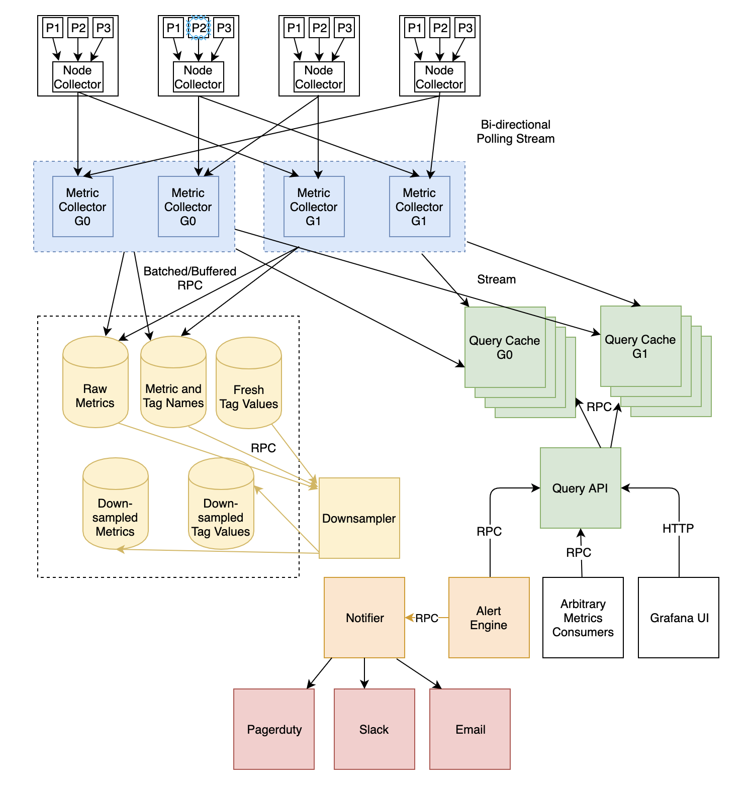
NodeCollector
Vortex metrics are stored in a ring buffer in each local process. In Vortex, the primary method of metric collection is poll-based and conducted on two tiers, with buffering on the second tier. The first tier is the NodeCollector. This is a process that runs on every node, responsible for polling the other processes of that node and aggregating the metrics into per-node totals. (We store both per-node and per-process stats, but the default query API only exposes per-node stats). The NodeCollector is in turn polled by a service called MetricCollector, which is responsible for writing the data to storage. NodeCollectors only poll the processes when they are themselves polled, which allows NodeCollector to be stateless, simplifying operations of this global service.
MetricCollector
Although the MetricCollector polls NodeCollectors every 10 seconds, internally it buffers the metrics for four minutes before flushing to storage. This buffering achieves two main purposes:
- It lets us remux the data streams—which allows data to enter in one arrangement and leave in another—to be grouped by metric name, rather than by node. When streaming data from the process through NodeCollector and into MetricCollector, it’s important for all data from a single node to be traveling together to ensure that the topology remains accurate. However, at query time it’s more useful to be able to sequentially read data from all nodes for a single metric, without reading unrelated data (other metrics).
- The buffering also substantially reduces write load on Cassandra, which Dropbox uses for the storage layer.
System-defined tags
We automatically tag each emitted metric with two additional tags that are universally useful.
- The first is the ID of the node that emitted this metric. In cases where the node corresponds to a physical hostname, we allow querying either by node_id or by tags derived from the node_id, such as datacenter, cluster, or rack. This sort of breakdown is very useful for troubleshooting problems caused by differences in networking throughput and connectivity, behavior differences across data centers and availability zones, etc.
- We also tag each metric with a "namespace," which is by default the name of the task that emitted this metric. This is useful when instrumenting core libraries such as Courier RPC, exception reporters, etc., since it allows filtering a specific service to just the core library metrics, without having to propagate extra logging information into all the libraries.
High availability
The MetricCollector service is actually split into two groups (G0 and G1 in the diagram above), and each NodeCollector establishes communication with a MetricCollector from each group. Each MetricCollector attempts to flush the data to storage if it’s not already there. This setup allows us to tolerate losing individual machines, with no interruption to service or data loss.
Limits
In order to provide a highly available ingestion pipeline, we’ve instituted limits in several places. Each node has a limited number of per-node and per-process metrics it can export, and metrics are dropped by the NodeCollector to comply with the limits. We have some heuristics in the drop algorithm to prioritize well-behaved users, such as preferential dropping of high-cardinality metric names (to protect Vortex users that deploy their code as part of the still-existing monolith we are moving away from). We also prefer metrics from processes that report fewer metrics over those that report more, to ensure that global services’ metrics aren’t dropped even if some application is misbehaving and exceeding limits.
Serving queries
The Vortex query subsystem consists of two services: the query cache and the query API. The query cache is partitioned and split into two groups (“G0” and “G1” in the diagram) for high availability, so the frontend exists to encapsulate the routing and make life simple for the clients.
Each query cache process consists of a live cache and a range cache. The live cache live-streams the results from the MetricCollectors, reducing query latency for real time alerting, while the range cache stores aggregated rows read from the storage tier.
Loading data
When the Vortex query service receives a request, the results of the query are typically already cached and up to date, so they can be served in milliseconds. However, sometimes the query has never been issued before or has been evicted from the cache; in these cases, it must be cold-loaded. Due to the ingestion setup and buffering done by MetricCollector, serving a non-cached query requires getting data from three sources:
- Load all relevant historical data from storage
- Load the unflushed data from MetricCollector (up to four minutes), as this data hasn’t been written to storage yet
- Register intent to receive streamed updates for the metrics used in the query with the MetricCollector. Once this is done, MetricCollectors will stream new data as it comes in, and the query system will keep the metric cached and up to date, so future queries will be cache hits.
The streaming is necessary because the most common use cases for querying metrics are auto-refreshing dashboards and alerts, both of which request the freshest data every few seconds.
Query language
While designing Vortex, we decided to implement our own query language, to cleanly represent system concepts such as topology. At a high level, the query language supports grouping by tag values, aggregating away tags, filtering tag values by regex, time shifting, and Unix-like function-chaining.
Some example queries and their explanation:
courier/client/requests[status]{server="vortex_query"}courier/server/requests[client]{_task="vortex_query", status!="success"} | top 5This query shows the five clients that are sending the most failing requests to the Vortex query service.
Topology joining
A join on a topology metric is specified by the @ operator. In a joined query, tags from both the topology metric and the main metric can be used interchangeably, as if they had all been reported on the same metric. To disambiguate them, tags originating from the topology are prefixed with an @ as well. For example:
courier/server/request_latency_ms[_p, @kernel]@node{_task="vortex_query", _p="p75|p95"}exception_log/exceptions[severity, @revision]@yaps{@service="vortex_query"} | per_secondMetric streaming
Since each query cache stores thousands of queries, it likely ends up receiving forwarded metric buckets from MetricCollectors on behalf of most of the nodes in the fleet. The following diagram represents the flow of data: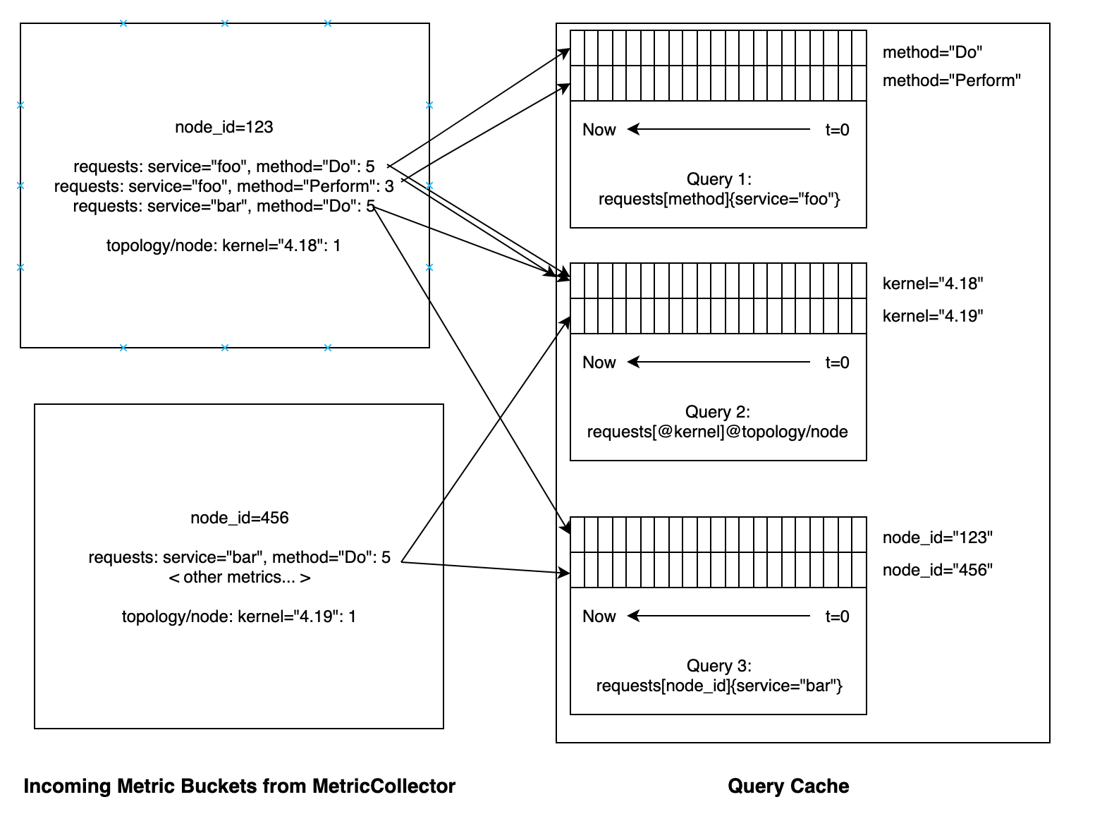
Query warmer
To take full advantage of the query caching, we run a service that prewarms queries that it finds on service dashboards. This ensures that when engineers open dashboards to investigate issues, their queries are served in milliseconds and they don't waste precious time waiting for data to load.Downsampling
As with any time-series database, Vortex performs downsampling of historical data as an optimization of performance and storage. Data is downsampled from 10-second granularity to 3 minutes, then 30 minutes, and finally 6 hours. We keep each lower granularity for progressively longer periods (six-hour data is retained forever), and at query time we choose a sampling rate such that we return a maximum of roughly 1,000 data points. This keeps the performance of queries roughly constant even as the time range is adjusted.Conclusion
In this post, we’ve described the design of our next-generation monitoring system. We’ve already scaled this system past the limits of the old system, and our users benefit from faster queries and higher trust in the system working correctly. We’ve successfully ingested more than 99.999% of reported buckets in the last few months, and our job orchestrator has replaced hundreds of failed hosts with no human intervention or disruption in service. In the next few months, we will continue to deliver new functionality and other improvements to our users, including recording rules, super-high cardinality metrics that can be selectively exported and persisted on the fly, integration with desktop and mobile client reporting libraries, a new metric type (a set cardinality estimator), and new query language features. With this work, we will continuously optimize our ability to gain insight into how our server applications (and downstream, our core products) are behaving.
Interested in joining us and working on Vortex or other interesting challenges? We’re hiring!


